Biohydrogen from Wastewater: Hybrid Fermentation-MEC-UASB Approach
Executive Summary
Biohydrogen from wastewater: Wastewater contains energy in its organic matter, measured as COD. Most treatment plants already recover a share of this energy as methane through anaerobic digestion. A three-stage hybrid process, acidification followed by a microbial electrolysis cell (MEC) and then a conventional UASB digester, can additionally recover part of this energy as hydrogen, a cleaner and higher-value fuel.
On a representative example plant, 1,000 cubic metres per day at 5,000 mg/L COD, the hybrid process produces about 83 kilograms of hydrogen per day in addition to methane.
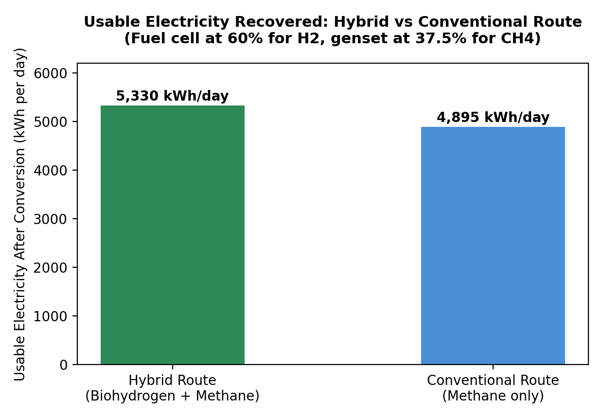
The total energy recovered is about 4% lower than a methane-only plant, but hydrogen converts to electricity far more efficiently in a fuel cell, so the hybrid process actually delivers about 9% more usable electricity.
The hybrid process needs higher capital investment, additional maintenance, and stricter hydrogen safety measures. Today it is best suited to pilot and demonstration projects rather than fully proven commercial installations.
1. Wastewater as an Energy Source
For decades, wastewater treatment has been viewed mainly as an environmental obligation, a process meant to remove pollutants before water is discharged or reused. While this remains its core purpose, wastewater is increasingly recognised as a source of recoverable resources, including energy, water, and nutrients.
The organic matter in wastewater carries significant chemical energy, commonly measured as Chemical Oxygen Demand (COD), the amount of oxygen required to oxidise the organic compounds present. In simple terms, COD indicates how much energy is stored in the wastewater’s biodegradable organic matter.
Traditionally, treatment plants have focused on removing this organic matter to meet environmental regulations. Modern plants increasingly aim to recover value from it before disposal, a shift that has given rise to the concept of the Water Resource Recovery Facility (WRRF), where wastewater is treated as a renewable resource rather than simply as waste.
Today, the most widely adopted method of energy recovery is anaerobic digestion, which converts part of the organic matter into methane rich biogas. The methane can generate electricity and heat, or be upgraded to biomethane as a renewable fuel. Thousands of municipal and industrial treatment plants worldwide already use this technology, making it a mature and commercially proven process.
Despite its success, conventional anaerobic digestion does not recover all the energy available in wastewater. A significant fraction remains in intermediate organic compounds or is lost during biological conversion. As global interest in renewable energy and the hydrogen economy grows, researchers have begun exploring ways to recover a greater share of this energy as hydrogen.
Hydrogen is attracting growing attention as a clean energy carrier with diverse applications. It can generate electricity in high efficiency fuel cells, serve as a feedstock for chemical industries, or replace fossil fuels in selected industrial processes. Recovering hydrogen directly from wastewater therefore offers a way to increase both the energy value and the economic return from existing treatment facilities.
The concept explored in this note is not to replace conventional methane production but to enhance it. By adding hydrogen recovery ahead of conventional anaerobic digestion, a plant can potentially produce both hydrogen and methane from the same organic load, two valuable renewable energy products, while still meeting the regulatory discharge standards the existing treatment process already achieves.
As wastewater treatment evolves from pollution control toward integrated resource recovery, technologies able to extract more value from the same stream will matter more. Biohydrogen production is one such opportunity. Although still at the pilot and demonstration stage, it offers a promising pathway to improve energy recovery, support decarbonisation, and turn wastewater treatment plants into renewable energy producers rather than energy consumers.
2. What Is Biohydrogen from Wastewater
Every wastewater treatment plant carries hidden energy in its organic matter, usually measured as COD. In most plants, this energy is recovered as methane through anaerobic digestion.
A newer approach recovers part of this energy as hydrogen instead. Hydrogen is a clean fuel with a high energy content per kilogram, and it can generate electricity more efficiently in a fuel cell than methane can in a gas engine.
Hydrogen produced from the organic matter in wastewater is called biohydrogen. Unlike green hydrogen, produced by splitting water using renewable electricity, or blue hydrogen, produced from natural gas with carbon capture, biohydrogen is generated directly from biodegradable organic matter. Because both the feedstock and the production process are different, biohydrogen is considered its own category of hydrogen.
Two main technologies are used to produce biohydrogen from wastewater:
- Dark Fermentation: a biological process carried out by naturally occurring bacteria.
- Microbial Electrolysis Cell (MEC): a process that combines biological activity with a small electrical input.
When used in sequence, these two technologies provide a practical way to recover hydrogen from industrial wastewater while still allowing the remaining organic matter to be converted into methane in a conventional anaerobic digester.
2.1 Why Hydrogen
Methane is already an effective energy source, but hydrogen offers several advantages. It produces only water when used in a fuel cell, converts energy to electricity more efficiently, and can also be used in chemical manufacturing or industrial fuel applications.
3. Two Engines of Biohydrogen
3.1 Dark Fermentation
Dark fermentation is a natural biological process that takes place without oxygen. Acid producing bacteria break down sugars and other easily biodegradable organic compounds, and the reactor is operated at a low pH so that the bacteria stop before producing methane.
As the bacteria digest the organic matter, they produce:
- Hydrogen gas
- Organic acids such as acetate and butyrate
No external electricity is required, since the bacteria provide all the energy the reaction needs. Dark fermentation works well with wastewater containing a high concentration of biodegradable organic matter, and it can also treat wastewater at relatively high loading rates.
The main limitation is that only a small portion of the available energy is converted into hydrogen. Most of the energy remains stored in the organic acids the process produces.
3.2 Microbial Electrolysis Cell (MEC)
A microbial electrolysis cell is an electrochemical reactor that uses bacteria together with a small electrical input to produce hydrogen. Inside the reactor, bacteria growing on the anode consume the organic acids produced during dark fermentation, and as they break these acids down they release electrons.
A small external voltage, much lower than that required for conventional water electrolysis, moves these electrons to the cathode, where they combine with hydrogen ions to produce hydrogen gas. Because of this electrical assistance, an MEC can produce three to four times more hydrogen per kilogram of COD than dark fermentation alone.
MECs perform best when fed wastewater rich in simple organic acids, which makes them an ideal second stage placed right after dark fermentation.
| Feature | Dark Fermentation | MEC |
| Driving force | Purely biological | Biological plus a small applied voltage |
| Typical hydrogen yield | 60 to 100 mL H2 per gram COD | 200 to 400 mL H2 per gram COD |
| Reactor throughput | High, comparable to standard high rate digesters | Low, limited by electrode surface area rather than reactor volume |
| Best feed | Raw, carbohydrate rich wastewater | Simple organic acids such as acetate |
| Maturity | Pilot to early demonstration | Laboratory to small pilot |
4. Why a Hybrid Makes Sense
Neither technology is sufficient on its own. Dark fermentation is fast and can treat large wastewater flows, but it converts only a small fraction of the available energy into hydrogen, with most of the energy remaining in the organic acids left behind. An MEC can recover much more hydrogen from these organic acids, but it cannot economically treat the entire wastewater flow, since its performance is limited by the available electrode surface area. Using both technologies in sequence lets each process do what it does best.
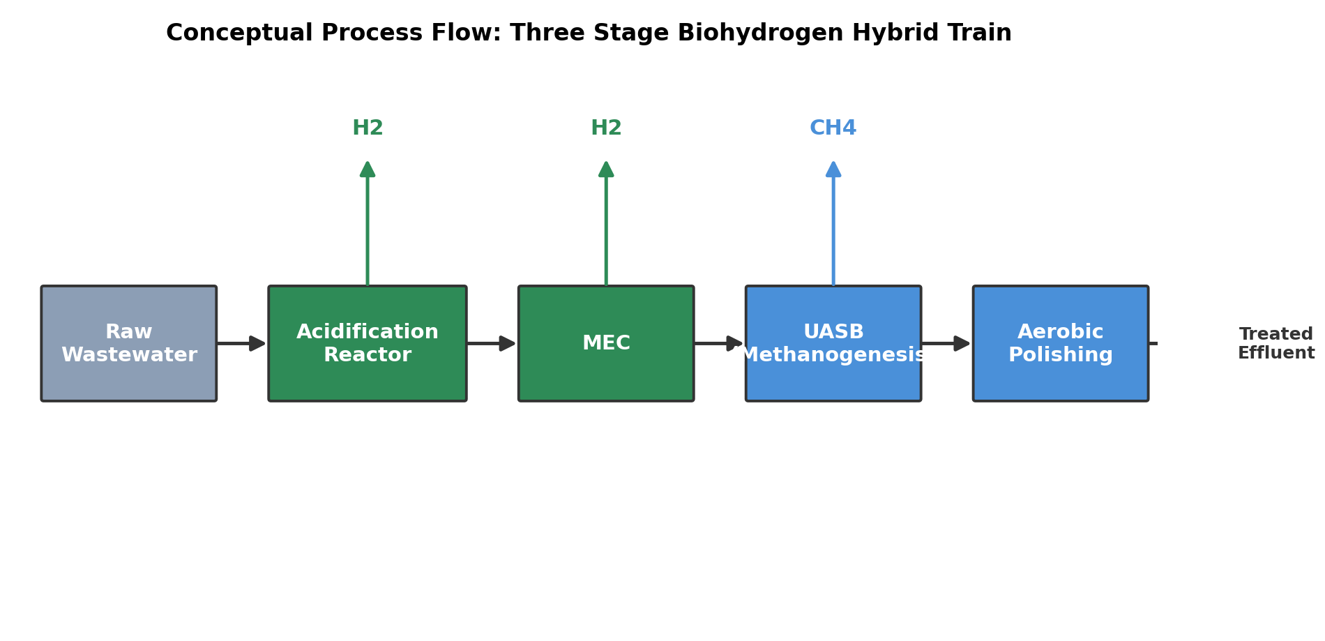
The wastewater passes through three stages:
- Acidification (dark fermentation): complex organic matter is converted into simple organic acids while producing the first portion of hydrogen.
- Microbial electrolysis cell: the organic acids are converted into additional hydrogen using a small electrical input.
- UASB digester: the remaining organic matter is converted into methane using conventional anaerobic digestion.
Any COD remaining after the UASB is removed in the plant’s existing aerobic treatment system before the treated water is discharged or reused.
This approach does not replace the conventional wastewater treatment process. Instead, it adds an extra hydrogen recovery step ahead of the existing anaerobic digestion stage, allowing the plant to recover more value from the same wastewater.
5. How Much COD Can Each Stage Handle
Each stage in the train has its own comfortable operating band, and the constraints behind each band are quite different.
| Stage | Comfortable COD range | Why this range applies |
| Acidification reactor | About 2,000 to 25,000 mg/L | Below this the acid forming bacteria are starved and grow too slowly; above it, acids build up faster than the system can buffer, and the pH crashes. |
| MEC | Works across a wide range, but current output plateaus once the anode surface is saturated | Hydrogen output depends on electrode surface area and on how well the wastewater conducts electricity, not on COD strength alone. Feeding it more COD than it can process is not harmful, the surplus simply passes through untouched to the next stage. |
| UASB (final polishing) | About 1,000 to 20,000 mg/L | Below this the granular sludge blanket that does the digestion can break down over time; above it, methane forming bacteria can be overwhelmed by acids or ammonia. |
The acidification reactor and the UASB must operate within their preferred COD ranges to stay stable. The MEC is more flexible, since it is limited by available electrode surface area rather than by COD concentration. If more COD enters the MEC than it can process, the excess is not wasted, it simply passes to the UASB, where it is converted into methane. Because of this, the process does not require dilution or recycle loops between the stages, the designer only needs to size the MEC correctly for the fraction of COD it should process.
6. A Worked Example
Consider an industrial wastewater treatment plant with the following characteristics:
- Flow: 1,000 cubic metres per day
- Influent COD: 5,000 mg/L
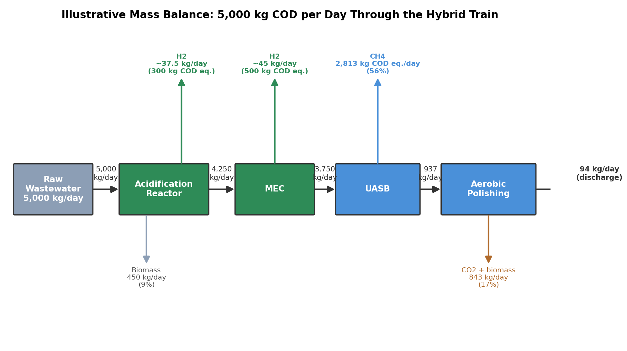
This corresponds to a total organic load of 5,000 kilograms of COD per day entering the treatment system.
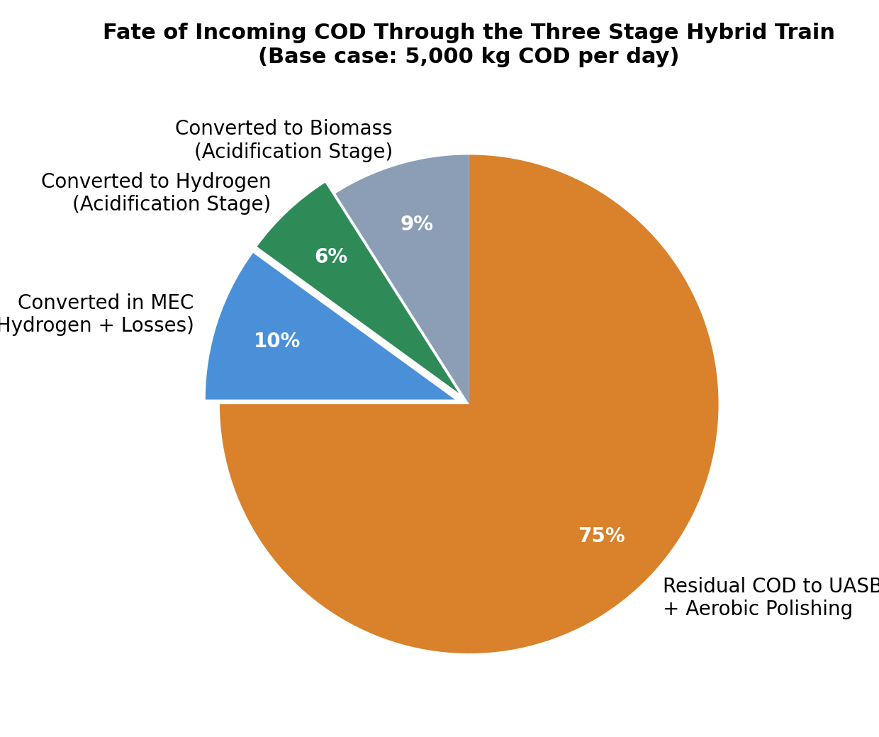
| Stream | COD (kg per day) | Share of feed |
| Incoming wastewater | 5,000 | 100% |
| Converted to biomass in acidification | 450 | 9% |
| Converted to hydrogen in acidification | 300 | 6% |
| Converted in the MEC (hydrogen plus losses) | 500 | 10% |
| Residual COD passed to UASB and aerobic polishing | 3,750 | 75% |
Carrying the balance through to discharge, the UASB removes most of the remaining COD as methane, and the final aerobic polishing step handles what is left, so the plant still ends with a compliant, low COD effluent, exactly as a conventional plant would.
For this example, the hybrid system produces approximately:
- Hydrogen: 83 kg per day
- Hydrogen volume: 917 Nm3 per day
- Hydrogen energy content: 2,767 kWh per day
Three quarters of the original COD load, 3,750 kilograms per day, still moves on to the UASB stage and then aerobic polishing before it can be safely discharged or reused. This is the part of the design that matters most for a bankable proposal: recovering hydrogen does not shorten or replace the treatment train a plant already needs, it adds an energy recovery step ahead of it.
7. Is the Trade Worth It
A fair comparison is between a conventional plant, where all COD is converted into methane, and a hybrid plant, where part of the COD is converted into hydrogen before the remaining COD is converted into methane.
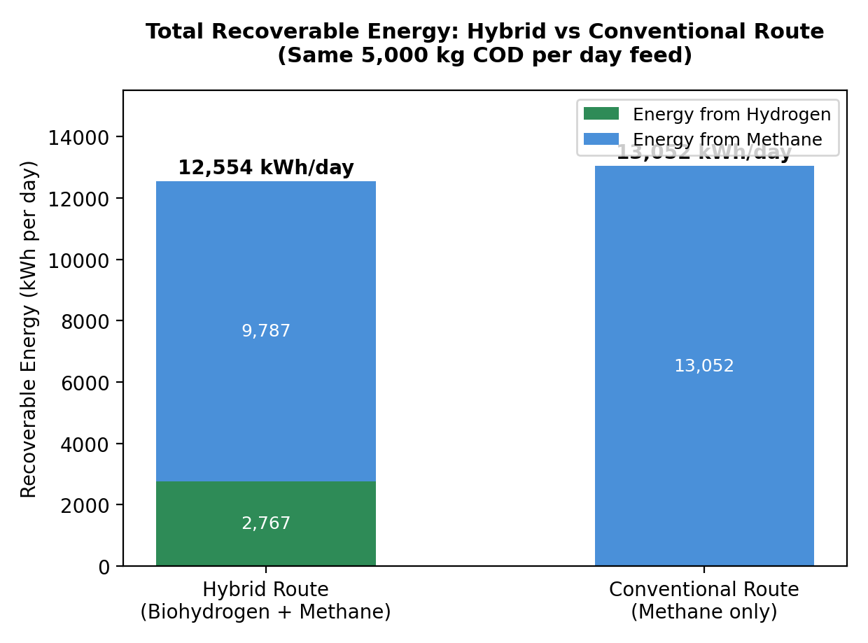
At first glance, the hybrid process appears to recover slightly less total energy. However, the quality of the recovered energy is higher.
About 22 % of the recovered energy is now available as hydrogen instead of methane. Hydrogen can generate electricity in a fuel cell at around 60 % efficiency, compared with 33 to 35 % efficiency for conventional combustion based generation, and typically 35 to 40 % for methane fired generator sets specifically.
As a result, the hybrid process delivers more usable electricity, even though the total energy recovered is slightly lower. The plant also now produces two marketable energy products, hydrogen and methane, instead of only methane, which creates operational flexibility and lets the operator target higher value energy markets where hydrogen demand exists.
A second useful comparison is how much external electrical energy each hydrogen generating route needs to produce a given amount of hydrogen, since this determines whether a technology is a net energy source or a net energy consumer.
| Route | External electricity needed per kg H2 | Where the rest of the energy comes from |
| Electrolysis of clean water | About 50 kWh per kg H2 | None, all the energy comes from the electricity supplied |
| MEC (wastewater fed) | About 10 kWh per kg H2 | Mostly from the organic content of the wastewater, only a small electrical push is needed |
| Dark fermentation | Effectively none | Entirely from the organic content of the wastewater |
Since a kilogram of hydrogen carries about 33.3 kilowatt hours of usable energy on a lower heating value basis, a constant published by the U.S. Department of Energy in its hydrogen storage technical targets, plain electrolysis of clean water is actually a net energy consumer, best understood as an energy storage method rather than an energy source. MEC and dark fermentation both draw most of their energy from the wastewater itself, which is what makes wastewater derived biohydrogen fundamentally different, and potentially more attractive, than electrolysis based hydrogen.
8. Environmental Performance and Carbon Benefit
The environmental benefit of the hybrid process is often misunderstood, so it is worth explaining correctly. The process does not reduce the total amount of carbon released from the wastewater.
The carbon in the incoming organic matter is conserved throughout the process. Eventually it is released as carbon dioxide, whether during acidification, during hydrogen production in the MEC, or when the methane produced in the UASB is finally used as fuel. The total carbon released stays almost the same as in a conventional biomethanation plant.
Why the Hybrid Process Avoids More Fossil CO2
Hydrogen can generate electricity in a fuel cell at around 60 % efficiency, while methane fired generators typically operate at 35 to 40 % efficiency. Although the hybrid process recovers slightly less total energy than a conventional methane only plant, it converts a larger share of that energy into usable electricity, so the plant can displace more grid or other fossil fuel based electricity than a conventional plant would have.
| Metric | Hybrid route | Conventional route |
| Usable electricity recovered | About 5,330 kWh per day | About 4,895 kWh per day |
| Assumed grid emission factor | 0.75 kg CO2 per kWh (illustrative) | 0.75 kg CO2 per kWh (illustrative) |
| Grid emissions avoided | About 4.0 tonnes CO2 per day | About 3.7 tonnes CO2 per day |
| Avoided emissions per year | About 1,460 tonnes CO2 per year | About 1,350 tonnes CO2 per year |
In this example, the hybrid process avoids approximately 110 additional tonnes of CO2 each year compared with a conventional methane only plant, an improvement of roughly 8 to 9 %, achieved solely because hydrogen converts its energy into electricity more efficiently.
9. Capex and Opex, the Added Cost Over Conventional Biomethanation
Adding hydrogen recovery is not free. The fair way to look at the cost is as an addition on top of a conventional biomethanation only plant of the same COD handling capacity, since the UASB and aerobic polishing stages a plant needs anyway do not go away.
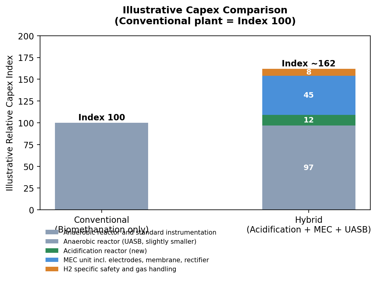
Using an indicative cost index, if the capital cost of a conventional biomethanation plant is taken as 100, the hybrid process typically falls between 160 and 170. Most of this increase comes from the microbial electrolysis cell, currently the most expensive part of the system. The acidification reactor uses conventional biological reactor technology and adds only a moderate cost, and hydrogen handling equipment such as gas detectors and dedicated piping contributes a relatively small additional investment. The UASB reactor may even be slightly smaller, since it receives a lower organic load after the hydrogen recovery stages.
Operating Cost (Opex)
The increase in operating cost is relatively modest compared with the increase in capital investment. The MEC needs a small electrical input to operate, low compared with conventional water electrolysis. The main operating cost uncertainty is electrode replacement, with a service life of roughly 3 to 5 years depending on operating conditions and electrode materials. The hybrid process is also more complex to operate, since it combines biological and electrochemical systems.
| Cost item | Conventional plant | Hybrid plant | Notes |
| Anaerobic reactor capex | Baseline (Index 100) | Slightly lower, since it handles less COD | UASB sized for residual COD only |
| Acidification reactor capex | Not applicable | Additional, illustratively 10 to 15 % of baseline | New unit, conventional reactor technology |
| MEC capex | Not applicable | Additional, illustratively 40 to 50 % of baseline | Dominant cost driver, expected to fall as the technology matures |
| Hydrogen safety and instrumentation capex | Standard biogas safety only | Additional, illustratively 6 to 10 % of baseline | Dedicated H2 detection, ventilation, segregated gas lines |
| Electricity opex | Baseline pumping and mixing load | Additional, roughly 450 kWh per day for the MEC in the worked example | Small compared with the capex impact |
| Electrode replacement opex | Not applicable | Recurring, typically every 3 to 5 years | Biggest source of opex uncertainty today |
| Operating complexity | One biological stage to manage | Three stages, biological and electrochemical, to monitor and balance | Calls for more skilled operator attention |
These figures are order of magnitude estimates meant to show where the added cost concentrates and how it is distributed, not a substitute for vendor quotations or a detailed project report. The largest cost component today is the MEC. As the technology matures, several factors are expected to reduce its cost:
- Lower cost electrode materials
- Improved manufacturing methods
- Higher production volumes
- Longer electrode life
- Better reactor designs
A similar trend has already been seen in case of many other technologies (e.g. Solar PV), where equipment costs have fallen significantly as the market has grown. Similar reductions are expected for MEC technology, but they have not yet been achieved at full commercial scale.
10. Hydrogen Handling, Safety Compared with Methane
Hydrogen is often described as a hazardous gas. A more accurate statement is that it presents different hazards from methane and therefore requires different engineering controls. Hydrogen can be handled safely, but only if the plant is designed specifically for its properties.
| Parameter | Hydrogen | Methane / biogas |
| Flammable range in air | About 4 to 75 % by volume, a very wide window | About 5 to 15 % by volume, a narrower window |
| Minimum ignition energy | About 0.017 millijoules, ignites very easily | About 0.28 millijoules, roughly 15 times higher |
| Flame visibility | Nearly invisible in daylight, harder to spot in an incident | Visible orange flame |
| Buoyancy and dispersion | Very light, rises and disperses fast outdoors, but can pool in ceiling pockets indoors | Also lighter than air, disperses somewhat more slowly, well understood in biogas practice |
| Natural odour for leak warning | None, needs dedicated hydrogen sensors | Biogas commonly carries a natural sulphide smell that gives early warning |
| Material compatibility | Can embrittle certain metals over long exposure, needs compatible piping and seals | No embrittlement concern, standard biogas materials are fine |
| Typical handling pressure | Often needs compression for storage or fuel cell use | Usually handled at low pressure, or moderately compressed if upgraded to CNG grade |
In practice this means the acidification and MEC stages need dedicated hydrogen gas detectors, distinct from the combustible gas detectors already used for biogas, along with good ventilation, flame arrestors, and gas lines kept separate from the methane lines until they reach a common utilisation point. None of this is exotic, the hydrogen and chemical process industries have decades of established practice for handling hydrogen safely, but it is a real addition to both the capex and the operating discipline of the plant, and it belongs squarely in the cost picture above rather than being treated as a minor afterthought.
11. Commercial Potential of Biohydrogen from Wastewater
Recovering hydrogen from wastewater offers a way to increase the value obtained from the same organic load. Instead of producing only methane, the plant can produce both hydrogen and methane, two marketable energy products from a single feedstock.
The technology should not be viewed as a replacement for conventional anaerobic digestion. It is an enhancement that adds hydrogen recovery while retaining the proven methane production process and the existing wastewater treatment train. The main benefits of the hybrid process are summarised below.
11.1 Two Energy Products from the Same Wastewater
A conventional anaerobic plant converts organic matter primarily into methane. The hybrid process converts part of the organic matter into hydrogen while the remaining COD continues to produce methane. This provides two potential revenue streams from the same wastewater and lets plant operators respond to changing energy prices and market demand.
11.2 Higher Value Energy Output
Although the hybrid process recovers slightly less total energy than a methane only system, hydrogen is a higher value energy carrier. Used in fuel cells, it converts chemical energy into electricity much more efficiently than methane fired generators, so the plant can produce more usable electricity from the same wastewater, improving overall energy utilisation.
11.3 Low External Energy Requirement
Unlike conventional water electrolysis, wastewater derived biohydrogen needs little external electricity. Dark fermentation uses only the energy already stored in the wastewater, and the MEC requires only a small electrical input, since most of the energy needed to produce hydrogen also comes from the wastewater. This significantly improves the overall energy balance of the process.
11.4 Minimal Impact on Existing Treatment Infrastructure
The hybrid process does not replace the existing wastewater treatment system. Instead, it introduces an additional hydrogen recovery stage ahead of the conventional UASB reactor. This means:
- Wastewater treatment performance is maintained
- Final effluent quality remains unchanged
- Existing biological treatment experience can still be used
- The technical risk of implementation is reduced
11.5 Growing Hydrogen Market
Demand for low carbon hydrogen is increasing worldwide. Potential applications include:
- Fuel cells
- Industrial heating
- Ammonia production
- Methanol production
- Refinery operations
- Steel manufacturing
- Hydrogen blending into natural gas networks where regulations permit
For facilities located close to hydrogen users, biohydrogen may become a valuable additional product rather than simply another source of electricity.
11.6 Current Limitations
Although the concept is technically sound, it should be presented realistically. Today, hybrid hydrogen recovery remains an emerging technology rather than a fully established commercial solution, and several challenges still need to be addressed before widespread industrial adoption.
Technology readiness. Dark fermentation has been demonstrated at pilot scale and is reasonably well understood. Microbial electrolysis cells, however, are still at the laboratory and pilot scale for most industrial wastewater applications, and large commercial installations remain limited.
Capital cost. The MEC currently represents the largest additional investment. Costs are expected to fall as manufacturing volumes increase and electrode technology improves, but current capital costs remain higher than those of conventional biomethanation.
Electrode life. Long term electrode durability remains one of the largest technical uncertainties. Industrial experience over many years of continuous operation is still limited, and improving electrode life will be essential for reducing operating costs and improving project economics.
Process complexity. The hybrid system combines biological and electrochemical processes. Compared with a conventional anaerobic digester, it requires:
- Additional instrumentation
- Closer process monitoring
- More sophisticated control systems
- Better trained operators
11.7 Overall Assessment
Based on current knowledge, the hybrid acidification, MEC, and UASB process represents a technically credible method of producing both hydrogen and methane from wastewater. Compared with conventional biomethanation, it offers:
- An additional renewable energy product
- Higher electricity recovery through fuel cells
- Greater flexibility in energy utilisation
- Improved fossil fuel displacement
- Access to emerging hydrogen markets
However, the technology has not yet reached the level of commercial maturity achieved by conventional anaerobic digestion.
12. Final Conclusion
Wastewater should no longer be viewed solely as a waste requiring treatment. It is also a valuable source of renewable energy and recoverable resources. Conventional anaerobic digestion has already shown how wastewater can produce methane and offset fossil fuel use. The addition of biohydrogen recovery extends this idea by generating a second, higher value energy product while preserving the proven treatment process. Although further commercial development is needed, the hybrid acidification, MEC, and UASB process offers a practical pathway toward more efficient resource recovery, greater energy flexibility, and improved sustainability.
For organisations seeking to move beyond wastewater treatment toward integrated resource recovery, biohydrogen represents a promising next step rather than a replacement for existing technology.
References
- S. Department of Energy, Hydrogen and Fuel Cell Technologies Office. Fuel Cells fact sheet and program pages, energy.gov/eere/fuelcells, source used in this note for the 60 % fuel cell efficiency figure and the 33 to 35% combustion-based generation comparison.
- International Energy Agency. Global Hydrogen Review 2025, IEA, Paris, iea.org/reports/global-hydrogen-review-2025, source used in this note for global hydrogen demand and low emissions hydrogen growth figures.
- Show, K. Y., Lee, D. J., Chang, J. S. Bioreactor and process design for biohydrogen production. Bioresource Technology, 2011.
- Logan, B. E., Call, D., Cheng, S., et al. Microbial electrolysis cells for high yield hydrogen gas production from organic matter. Environmental Science and Technology, 2008.
- Kadier, A., Simayi, Y., Abdeshahian, P., et al. A comprehensive review of microbial electrolysis cells as a platform technology for hydrogen production and wastewater treatment. Alexandria Engineering Journal, 2016.
- Guo, X. M., Trably, E., Latrille, E., et al. Hydrogen production from agricultural waste by dark fermentation, a review. International Journal of Hydrogen Energy, 2010.
- Cheng, S., Logan, B. E. Sustainable and efficient biohydrogen production via electrohydrogenesis. Proceedings of the National Academy of Sciences, 2007.
- Kothari, R., Singh, D. P., Tyagi, V. V., Tyagi, S. K. Fermentative hydrogen production, an alternative clean energy source. Renewable and Sustainable Energy Reviews, 2012.
- Central Electricity Authority, Government of India. CO2 Baseline Database for the Indian Power Sector, User Guide, latest edition.
- Intergovernmental Panel on Climate Change. Guidelines for National Greenhouse Gas Inventories, treatment of biogenic carbon.
- Metcalf and Eddy, revised by Tchobanoglous, G., Stensel, H. D., Tsuchihashi, R., Burton, F. Wastewater Engineering, Treatment and Resource Recovery. McGraw Hill.
- National Fire Protection Association. NFPA 2, Hydrogen Technologies Code, guidance on hydrogen flammability and safe handling.
Figures used in the worked example are illustrative, built from typical ranges reported in the literature above, and are meant to show the shape of the mass and energy balance rather than to substitute for site specific testing.
Normalised Biogas Yield
Raw biogas production volume is the most commonly monitored gas-phase parameter in operating digester, and the least sensitive early warning indicator available. A system can accumulate VFAs sufficient to drive the VFA/alkalinity ratio above 0.4 while total gas production declines by only 10–15%. Normalised biogas yield removes the masking effect of loading variation and reveals methanogenic efficiency directly.
What Normalised Biogas Yield Measures
Normalised biogas yield is the volume of biogas produced per unit of organic matter removed, expressed as m³ of biogas per kg of COD removed. The word ‘normalised’ means that the effect of organic loading variability has been removed: if loading increases and gas production increases proportionally, the yield is unchanged. If loading increases but gas production does not keep pace, the yield declines, signalling that methanogenic efficiency is falling.
It is the equivalent of measuring fuel efficiency in kilometres per litre rather than total kilometres driven. Total kilometres tells you how far you went. Kilometres per litre tells you how efficiently the engine is performing.
The Calculation
| Step | Formula / Value |
|---|---|
| COD removed (kg/day) |
[Influent COD (mg/L) − Effluent COD (mg/L)] × Flow rate (m3/day) ÷ 1,000 |
| Normalised biogas yield |
Total biogas produced (m3/day) ÷ COD removed (kg/day) |
Worked Example
| Parameter | Value |
|---|---|
| Influent COD | 8,000 mg/L |
| Effluent COD | 1,200 mg/L |
| COD removed | 6,800 mg/L |
| Flow rate | 500 m3/day |
| COD removed per day | 6,800 × 500 ÷ 1,000 = 3,400 kg/day |
| Biogas produced | 2,040 m3/day |
| Normalised biogas yield | 2,040 ÷ 3,400 = 0.60 m3/kg COD removed |
Benchmark Values and Their Interpretation
Theoretical maximum biogas yield from COD removal is approximately 0.35 m³ methane per kg COD at standard conditions. For total biogas at 60–65% methane content, the equivalent yield is approximately 0.50–0.65 m³ per kg COD in a well-operated system.
| Normalised Yield (m3/kg COD removed) | What It Indicates |
|---|---|
| 0.55 – 0.65 | Healthy system — methanogenesis efficient |
| 0.45 – 0.55 | Moderate efficiency — investigate VFA accumulation or temperature |
| 0.35 – 0.45 | Poor efficiency — methanogenic activity significantly below potential |
| Below 0.35 | Serious underperformance — active biological disturbance likely |
These ranges vary with wastewater composition: lipid-rich wastewaters produce more methane per kg COD than carbohydrate-rich ones. The plant’s own historical baseline is therefore more meaningful than generic benchmarks — the trend matters more than the absolute value.
Why It Detects Problems That Raw Gas Volume Misses
Consider two scenarios that appear identical on a raw gas flow meter but represent opposite biological realities:
| Scenario | Raw Gas Volume | Normalised Yield | What Is Actually Happening |
|---|---|---|---|
| A: Loading up 20%, gas up 15% | Looks acceptable — flow increasing | Dropped from 0.60 to 0.53 | VFAs accumulating; system under early methanogenic stress masked by loading increase |
| B: Loading down 20%, gas down 20% | Looks alarming — flow decreasing | Stable at 0.61 | Biology healthy; production lower because less substrate available |
Without normalisation, Scenario A looks acceptable and Scenario B looks worrying. With normalisation, the reality is exactly reversed. Raw gas volume without normalisation is a loading signal, not a performance signal.
How to Implement It
The required data is already available in every plant measuring influent COD, effluent COD, flow rate, and gas production. The calculation takes two minutes per week from a simple spreadsheet. Plot the result as a weekly trend line alongside the VFA/alkalinity ratio and OLR.
A downward trend in normalised yield sustained over three to four consecutive weeks — even if absolute gas production appears stable or rising because loading is increasing — is the signal to measure VFA/alkalinity ratio more frequently and investigate whether methanogenic efficiency is declining. The yield trend will typically show the problem 2–3 weeks before the VFA/alkalinity ratio reaches an intervention threshold.
Divergence Between OLR and Normalised Yield — The Critical Pattern
The most diagnostically significant pattern is a divergence between organic loading rate (OLR) and normalised yield: loading increasing or stable, yield declining. This indicates that the methanogenic community is not keeping pace with the organic load being applied — the biological gap that, if not identified and corrected, proceeds to VFA accumulation and eventual acidification.
| OLR Trend | Normalised Yield Trend | Interpretation | Action |
|---|---|---|---|
| Stable | Declining | Methanogenic efficiency falling — loading unchanged |
Investigate temperature, nutrients, pH; increase VFA/alk measurement frequency |
| Increasing | Declining | Methanogenic population cannot keep pace with load |
Reduce OLR increase rate; verify sludge inventory; check SRT |
| Increasing | Stable | System absorbing additional load efficiently |
Monitor; continue planned loading increase |
| Declining | Increasing | Load reduction improving methanogenic performance |
Positive signal; biology recovering |
What Operators Should Do
- Calculate normalised biogas yield regularly using COD removed rather than only total gas generated.
- Correct gas volume to standard conditions (Nm³) for meaningful comparison.
- Trend gas yield daily, weekly, and monthly to identify gradual deterioration.
- Investigate declining methane yield even if total gas volume appears stable.
- Check gas flowmeter calibration and sensor reliability periodically.
- Avoid increasing feed solely because total gas production rises temporarily.
- Monitor VFA trends when gas efficiency starts declining.
References
- Schievano, A. et al. (2014). Toward a predictive model of biodegradability and biogas production potential in anaerobic digestion. Energy & Fuels, 28(8), 5243–5250.
- Angelidaki, I. et al. (2009). Defining the biomethane potential (BMP) of solid organic wastes and energy crops: a proposed protocol for batch assays. Water Science & Technology, 59(5), 927–934.
- Melse, R.W. & Timmerman, M. (2009). Sustainable intensive livestock production demands manure and exhaust air treatment technologies. Bioresource Technology, 100(22), 5506–5511.
- Lossie, U. & Pütz, P. (2008). Targeted control of biogas plants with the help of FOS/TAC. Practice Report, Hach-Lange GmbH.
- Batstone, D.J. et al. (2002). Anaerobic Digestion Model No. 1 (ADM1). IWA Publishing, London.
- Green Pulse™ Anaerobic Treatment Module — Internal Technical Documentation (2024).
VFA/Alkalinity Ratio and Biogas Composition Monitoring
The VFA/alkalinity (FOS/TAC) ratio is the most sensitive daily early warning parameter for anaerobic process stability. Online biogas composition monitoring — CH₄, CO₂, H₂, and H₂S — complements it with continuous real-time resolution. Together they provide a warning window of 12–24 hours ahead of pH decline. pH, by contrast, is the last indicator to move and the least useful for early intervention.
The VFA/Alkalinity Intervention Hierarchy
| Ratio Range | System Status | Required Actions |
|---|---|---|
| Below 0.3 (stable) | Healthy | Monitor daily. Trend OLR and normalised biogas yield alongside ratio. |
| Below 0.3 (trending up 3+ days) | Early warning |
Investigate: (a) OLR increase; (b) temperature drop; (c) nutrient imbalance. Increase measurement to twice daily. |
| 0.3 – 0.4 | Active stress |
Reduce OLR 15–20%. Check N and P dosing. Verify temperature. Add NaHCO3 if alkalinity below 2,000 mg/L. Increase recirculation if below design maximum. |
| 0.4 – 0.5 | Serious distress — acetogenesis compromised |
Reduce OLR 30–40% immediately. Add alkalinity aggressively. Check GC-VFA speciation: propionate and butyrate accumulation indicates acetogenic inhibition in addition to methanogenic. Assess methanogenic activity. |
| Above 0.5 | Emergency |
Halt or severely curtail feed. Maintain temperature and mixing. Add NaHCO3 at 1–2 kg/m3 reactor volume/day. Source external sludge for seeding. Accept 4–10 weeks recovery minimum. |
What Biogas Composition Tells You
Biogas from a healthy digester is typically 60–70% CH₄ and 30–40% CO₂, with trace H₂S, nitrogen, and hydrogen. These proportions are a direct reflection of the metabolic activity of all four digestion stages simultaneously — and they change in predictable ways when the system is stressed.
Methane Percentage — The Primary Health Indicator
Methane is produced exclusively by methanogens. A sustained decline in CH₄ percentage of more than 3–4 percentage points over 24–48 hours — from a stable 65% to 61–62% — in the absence of a known loading change is a reliable early indicator of methanogenic stress. When CH₄ declines while total gas flow is stable or rising, the CO₂ fraction is increasing to compensate — CO₂ production from acidogenesis and acetogenesis continues while methanogenic conversion lags. An operator monitoring only the gas flow meter will see nothing unusual. An operator monitoring gas composition will see the warning.
Carbon Dioxide Percentage — The Alkalinity Signal
CO₂ in biogas exists in equilibrium with dissolved CO₂ and bicarbonate. As VFAs accumulate and consume bicarbonate alkalinity, more CO₂ partitions into the gas phase. A sustained increase in CO₂ percentage alongside stable or declining CH₄ is the gas-phase signature of alkalinity stress — providing a continuous signal complementing the once-daily VFA/alkalinity ratio.
Hydrogen — The Acetogenic Stress Indicator
Hydrogen in biogas is normally below 100 ppm. When methanogenic activity is suppressed, hydrogen consumption slows, partial pressure rises, and acetogenic reactions become thermodynamically unfavourable — causing propionate and butyrate accumulation even before acetate concentrations have risen significantly. H₂ above 200 ppm indicates active acetogenic inhibition. Above 500 ppm, propionate and butyrate are accumulating in the liquid phase. Above 1,000 ppm, severe methanogenic inhibition is present and the VFA/alkalinity ratio is almost certainly above 0.4 and rising. The hydrogen signal precedes the VFA/alkalinity ratio by 12–24 hours — but only if it is being measured.
Hydrogen Sulphide — The Inhibition and Corrosion Indicator
H₂S originates from sulphate reduction by sulphate-reducing bacteria (SRB) — a fifth microbial community that competes with methanogens for acetate and hydrogen when sulphate is present in the feed. Rising H₂S percentage without a change in influent sulphate indicates that SRBs are gaining a larger share of available substrate — a secondary indicator of methanogenic suppression, particularly in sulphate-bearing pharmaceutical, chemical, and food processing effluents. H₂S above 500 ppm also accelerates corrosion of gas piping, engines, and heat exchangers.
Recirculation: What It Can and Cannot Do
Recirculation dilutes incoming feed with alkalinity-rich reactor liquor, buffers influent VFA concentration and pH, and dilutes inhibitory compounds. It does not create alkalinity. If total system alkalinity is being consumed by VFA accumulation faster than it is being replenished by methanogenic activity, recirculation redistributes what remains but does not arrest the decline.
Plants that treat recirculation as a primary management response to a rising VFA/alkalinity ratio typically experience a series of progressively more severe acidification events, each starting from a lower alkalinity reserve, until the methanogenic population is too depleted to sustain operation without external sludge seeding. Recirculation is a buffer management tool for transient disturbances in a biologically healthy system — not a corrective tool for a system in biological decline.
Integrated Monitoring Framework
| Parameter | Frequency | What It Detects First | Limitation |
|---|---|---|---|
| Biogas H2 (online) | Continuous | Acetogenic/methanogenic stress onset (12–24 hr ahead of VFA ratio) | Requires dedicated H2 sensor |
| CH4 % (online) | Continuous | Methanogenic activity decline | Lags H2 by several hours |
| CO2 % (online) | Continuous | Alkalinity consumption | Can be masked by OLR variation |
| H2S (online) | Continuous | SRB competition; sulphide equilibrium shift | Indirect methanogenic stress indicator |
| VFA/alkalinity ratio (lab) | 1–2× daily | Accumulated liquid-phase imbalance | No real-time resolution |
| Normalised biogas yield | Weekly | Long-term methanogenic efficiency drift | Lags acute events by days |
| pH (online) | Continuous | Advanced alkalinity exhaustion | Last line of defence — too late for easy intervention |
The most robust early warning system for an industrial anaerobic reactor combines at minimum three parameters: online CH₄/CO₂ monitoring, daily VFA/alkalinity measurement, and weekly normalised yield tracking. For plants with high-value biogas production or high-consequence compliance requirements, adding online H₂ monitoring provides a 12–24 hour earlier warning window that can make the difference between a managed load reduction and an emergency shutdown.
What Operators Should Do
- Calculate gas yield per kg COD removed regularly.
- Correct gas volume to normalised conditions (Nm³).
- Investigate declining methane yield immediately.
- Validate gas flowmeter calibration periodically.
- Use trend analysis to identify gradual biological deterioration before process upset occurs.
References
- Lossie, U. & Pütz, P. (2008). Targeted control of biogas plants with the help of FOS/TAC. Practice Report, Hach-Lange GmbH.
- Boe, K. et al. (2010). Online headspace chromatographic method for measuring VFAs in anaerobic digesters. Water Science & Technology.
- Hickey, R.F., Vanderwielen, J., & Switzenbaum, M.S. (1989). The effect of heavy metals on methane production and hydrogen and carbon monoxide levels during batch anaerobic sludge digestion. Water Research.
- Ahring, B.K., Sandberg, M., & Angelidaki, I. (1995). Volatile fatty acids as indicators of process imbalance in anaerobic digestors. Applied Microbiology and Biotechnology.
- van Lier, J.B. (2008). High-rate anaerobic wastewater treatment: diversifying from end-of-the-pipe treatment to resource-oriented conversion techniques. Water Science & Technology.
- Green Pulse™ Anaerobic Treatment Module — Internal Technical Documentation (2024).
Recovering a Sour Anaerobic Digester
Recovery from a sour anaerobic digester is governed by the growth kinetics of the slowest organisms in the process — aceticlastic methanogens with doubling times of 3–30 days. Understanding the population mathematics prevents the two most common management errors: reintroducing feed too early, and underestimating how long recovery genuinely requires.
Start Recovery on Accumulated VFAs — Not Fresh Feed
Before detailing recovery timelines, it is important to recognise a significant and frequently underutilised advantage: fresh feed is not needed to begin rebuilding the microbial population. The accumulated VFAs already present in the reactor — often representing several days’ worth of organic loading — serve as an abundant and immediately bioavailable carbon and energy source for both methanogens and acetogens.
Recovery should therefore begin at zero or severely reduced feed input, allowing the microbial population to grow on the existing VFA pool after pH has been corrected through alkalinity addition. Introducing fresh feed before the accumulated VFA pool has been substantially consumed simply adds to the organic acid load, prolongs inhibitory conditions, and extends the recovery period.
Ongoing Methanogen Losses During Recovery
Even during the recovery phase, methanogen losses continue through three routes. For a representative 1,000 m³/day pharmaceutical wastewater plant treating 5,000 mg/L COD at 85% removal: total reactor sludge inventory ~8,000–10,000 kg VSS; methanogenic fraction 10–20% = 800–2,000 kg VSS at steady state.
| Loss Route | Basis | Methanogen Fraction | Daily Methanogen Loss |
|---|---|---|---|
| Effluent overflow (VSS at 100 mg/L) | 100 kg VSS/day total | 10–20% | 10–20 kg VSS/day |
| Deliberate sludge wastage (0.5–1.0% of inventory) | 40–100 kg VSS/day total | 10–20% | 8–10 kg VSS/day |
| Die-off from residual pH / toxicity | Variable | — | 5–20 kg VSS/day (recovery phase) |
| Total ongoing methanogen loss | — | — | 18–50 kg VSS/day |
Recovery Timeline Projections
Under normal operating conditions with no acidification stress, net methanogen accumulation is approximately 80–100 kg VSS/day, representing ~0.8–1.0% of total sludge inventory per day. Building the methanogenic population by 20% from a depleted but non-acidified state therefore takes approximately 20–25 days. In a fully soured system where aceticlastic methanogens have been severely depleted and pH correction is still in progress, this timeline extends substantially.
| Recovery Stage | Typical Duration | Key Actions |
|---|---|---|
| pH correction and acid neutralisation | 2–5 days | NaHCO3 at 1–2 kg/m³/day; hold feed at zero or minimum |
| VFA drawdown on accumulated pool | 3–7 days | Maintain temperature; minimal feed; monitor CH4% daily |
| Initial methanogen recovery (VFA ratio 0.3–0.4) | 7–14 days | Resume feed at 10–15% of design; increase in 10% steps |
| Full methanogen repopulation | 20–60+ days | Step feed to 100%; achieve normalised biogas yield baseline |
Where the methanogenic inventory is estimated below 30% of steady-state, sourcing external granular sludge for seeding is the single most effective intervention — it typically halves recovery time by providing an immediate inoculum of active aceticlastic methanogens already adapted to the wastewater characteristics.
Step-by-Step Recovery Protocol
Step 1 — Stabilise pH (Days 1–5)
Stop or severely curtail feed. Add sodium bicarbonate (NaHCO₃) at 1–2 kg per m³ of reactor volume per day, not caustic soda, which creates localised pH spikes that damage the remaining methanogenic population. Target pH 6.8–7.2. Maintain temperature and mixing continuously. Important to net, the NaHCO₃ requirement depends on VFA load, buffering deficit, and reactor alkalinity.
Step 2 — Confirm Stability Before Feed Resumption
Do not resume feed until: (a) VFA/alkalinity ratio is below 0.3 on two consecutive daily measurements; (b) biogas methane percentage is recovering toward 55–60%; (c) effluent pH is stable at 7.0±0.2. Meeting all three criteria simultaneously before feeding prevents the most common recovery failure mode — premature feed reintroduction re-acidifying a partially recovered system.
Step 3 — Feed Stepwise, Not Gradually
Resume feed in discrete steps of 10–15% of design load, with a minimum hold of 2–3 days between each increment. At each hold point, verify that the VFA/alkalinity ratio is stable or declining before proceeding. If the ratio rises at any step, hold or reduce; do not continue loading upward.
Step 4 — Supplement with External Sludge If Required
If VFA/alkalinity ratio is not declining after 7–10 days despite pH correction and zero feed, or if methane percentage is not recovering, the methanogenic population is likely below the threshold for self-recovery at a meaningful rate. Source granular sludge from an operating UASB treating a similar substrate. Seed at 5–10% of reactor volume.
Note: bioaugmentation rarely overcomes poor root-cause correction.
Common Recovery Failures
| Failure Mode | Cause | Prevention |
|---|---|---|
| Re-acidification 7–14 days into recovery | Feed resumed before VFA/alk ratio < 0.3 | Apply all three stability criteria before feeding |
| Ratio declines but plateaus at 0.35–0.40 | Methanogenic population too small to accelerate | Source external sludge; extend zero-feed period |
| Temperature fluctuation during recovery | Loss of heating/mixing during recovery phase | Maintain temp ±1°C; never reduce mixing |
| pH overcorrection (>7.8) | Caustic soda dosing; overdose of NaHCO3 | Use NaHCO3 only; dose incrementally with daily monitoring |
References
- van Lier, J.B., Mahmoud, N., & Zeeman, G. (2008). Anaerobic wastewater treatment. In: Biological Wastewater Treatment: Principles, Modelling and Design. IWA Publishing.
- Lettinga, G. (1995). Anaerobic digestion and wastewater treatment systems. Antonie van Leeuwenhoek.
- Speece, R.E. (1996). Anaerobic Biotechnology for Industrial Wastewaters. Archae Press, Nashville.
- Batstone, D.J. et al. (2002). Anaerobic Digestion Model No. 1 (ADM1). IWA Publishing, London.
- Ahring, B.K. (1994). Status on science and application of thermophilic anaerobic digestion. Water Science and Technology.
- Green Pulse™ Anaerobic Treatment Module — Internal Technical Documentation (2024).
Diagnosing a Sour Anaerobic Digester
When an anaerobic digester sours, the first and most important task is not to begin recovery; it is to accurately diagnose which microbial pathways have been damaged and to what degree. Rushing into recovery protocols without this diagnosis is one of the most common causes of failed or prolonged restarts.
Why VFA Speciation by GC Matters
The single most informative test during a sour digester assessment is a full VFA speciation profile by gas chromatography (GC), not simply a total VFA or alkalinity measurement. The ratio and absolute concentrations of individual VFAs — acetic, propionic, butyric, isobutyric, valeric, and isovaleric acids, reveal which microbial group has failed and how severely.
A total VFA result tells you something is wrong. GC speciation tells you where the process has broken down and what is still functioning, enabling a targeted recovery strategy rather than generic alkalinity addition and load reduction.
Diagnostic Logic — Reading the VFA Profile
| VFA Pattern Observed | Pathway Implicated | Severity |
|---|---|---|
| Acetate dominant; propionate low; total VFA 500–2,000 mg/L | Aceticlastic methanogenesis inhibited only; acetogens still functioning | Moderate |
| Acetate very high (>2,000 mg/L); still dominant VFA species | Aceticlastic methanogenesis severely depleted | Severe |
| Propionate elevated (>500 mg/L); propionic:acetic ratio >0.5 | Syntrophic acetogenesis of propionate impaired; H₂ partial pressure rising | Moderate–Severe |
| Propionic:acetic ratio >1.0 | Acetogenesis collapsed; hydrogenotrophic methanogens also failing | Severe |
| Butyrate + propionate both >500 mg/L simultaneously | Full acetogenic pathway breakdown; H₂ partial pressure critically elevated | Severe |
| Isobutyrate, valeric, isovaleric above baseline | Fermentation stage dysregulated; amino acid catabolism pathways disrupted | Severe / Complex |
The Propionic:Acetic Ratio — A Critical Diagnostic Threshold
In a digester that has suffered only aceticlastic methanogen inhibition, the propionic:acetic ratio remains low. Acetate accumulates but propionate does not, because acetogens are still active and converting propionate to acetate (even if methanogens cannot consume it fast enough). When this ratio exceeds 0.5 — and especially when it exceeds 1.0 — it signals that hydrogen partial pressure has risen high enough to thermodynamically block syntrophic propionate oxidation.
A propionic:acetic ratio below 0.3 in a sour digester typically indicates methanogenic failure only — a difficult but manageable recovery. Above 0.5, acetogenesis is compromised. Above 1.0, the acetogenic pathway has effectively collapsed and recovery will require weeks, not days.
Supporting Parameters — Full Diagnostic Framework
| Parameter | Method | Result Pattern | Pathway Implicated | Severity |
|---|---|---|---|---|
| Acetic acid | GC-FID | 500–2,000 mg/L; dominant VFA | Aceticlastic methanogenesis inhibited | Moderate |
| Acetic acid | GC-FID | >2,000 mg/L; dominant | Aceticlastic methanogenesis severely depleted | Severe |
| Propionic acid | GC-FID | >500 mg/L; ratio >0.5 | Syntrophic acetogenesis impaired | Moderate–Severe |
| Propionic acid | GC-FID | >1,500 mg/L; ratio >1.0 | Acetogenesis collapsed; H₂-trophic methanogens failing | Severe |
| Butyric acid | GC-FID | Mildly elevated + acetate | Early-stage acetogenic inhibition | Mild–Moderate |
| Butyric + propionic both >500 | GC-FID | Both simultaneously elevated | Full acetogenic pathway breakdown | Severe |
| Isobutyric / valeric / isovaleric | GC-FID | Above baseline | Fermentation stage dysregulated | Severe / Complex |
| Biogas CH₄ content | Gas analyser | <50% (normal 60–70%) | Active methanogenesis suppressed | Moderate–Severe |
| Biogas CH₄ content | Gas analyser | <30% or CO₂ dominant | Methanogenesis near collapse | Critical |
| FOS/TAC ratio | Titration | >0.4 | Imbalance; instability warning | Moderate |
| FOS/TAC ratio | Titration | >0.8 | Severe imbalance; active distress | Severe |
| H₂ partial pressure | H₂ probe / GC | >10−4 atm | Acetogenesis thermodynamically unfavourable | Severe |
The Acetogenesis Bottleneck — A Frequently Missed Complication
Acetogens can only convert propionate and butyrate to acetate and hydrogen when hydrogen partial pressure is kept very low — a condition maintained by hydrogenotrophic methanogens. When methanogenic activity is suppressed, hydrogen accumulates and acetogenesis becomes thermodynamically unfavourable regardless of acetogen population size.
During recovery, even as aceticlastic methanogenesis begins to partially recover and acetate consumption resumes, propionate and butyrate continue to accumulate if hydrogenotrophic methanogen activity remains insufficient. The effluent VFA profile characteristically shifts from acetate-dominated to propionate- and butyrate-dominated — a clear indicator that the system is in combined acetogenic and methanogenic distress, and that recovery will take longer than a simple methanogen reactivation timeline would suggest.
What Operators Should Do
- Monitor VFA speciation where possible.
- Trend propionic acid separately.
- Interpret pH together with alkalinity and methane.
- Avoid aggressive loading increases during stress.
- Investigate declining methane percentage immediately.
References
- Ahring, B.K., Sandberg, M., & Angelidaki, I. (1995). Volatile fatty acids as indicators of process imbalance in anaerobic digestors. Applied Microbiology and Biotechnology, 43(3), 559–565.
- Pullammanappallil, P.C. et al. (2001). Stable performance of anaerobic digestion in the presence of a high concentration of propionic acid. Bioresource Technology, 78(2), 165–169.
- Batstone, D.J. et al. (2002). Anaerobic Digestion Model No. 1 (ADM1). IWA Publishing, London.
- Lossie, U. & Pütz, P. (2008). Targeted control of biogas plants with the help of FOS/TAC. Practice Report, Hach-Lange GmbH.
- Boe, K. et al. (2010). Online headspace chromatographic method for measuring VFAs in anaerobic digesters. Water Science & Technology, 61(11), 2729–2736.
- Green Pulse™ Anaerobic Treatment Module — Internal Technical Documentation (2024).
Two-Stage Reactor Design
The most effective engineering response to the kinetic asymmetry between anaerobic digestion stages is a design that physically separates the fast-growing acidogenic communities from the slow-growing methanogenic and acetogenic communities, and provides each with the retention time, pH environment, and sludge management strategy it actually needs.
The Two-Stage Process — Separating the Four Biochemical Stages
The most robust design response to the kinetic asymmetry between hydrolysis/acidogenesis and acetogenesis/methanogenesis is a two-reactor configuration.
Reactor 1 — Acidogenic Reactor
Designed to maximise hydrolysis and acidogenesis. Operates at pH 5.5–6.5 — below the methanogenic tolerance range — which prevents methanogenic colonisation and keeps the community composition clean. Short HRT and frequent sludge wasting based on VSS concentration. Because acidogens double in 1–2 hours, aggressive wasting does not risk population collapse. The effluent from Reactor 1 is a VFA-rich, consistent stream — an ideal and predictable feed for the methanogenic reactor.
Reactor 2 — Methanogenic Reactor
Designed to maximise aceticlastic methanogenesis and syntrophic acetogenesis. Operates at pH 6.8–7.4. Extended HRT. Minimal, precisely calculated daily sludge wasting based on measured VSS and target SRT — typically 20–60 days. Because complex organic substrate has been removed in Reactor 1, acidogens cannot colonise Reactor 2. The biomass becomes progressively enriched in methanogens and acetogens, and the aceticlastic methanogen fraction typically reaches 2–3 times the concentration achievable in an equivalent single-stage system.
The Sludge Management Advantage of Two-Stage Design
In a single-stage reactor, sludge wasting decisions are a compromise between the needs of all four communities simultaneously. Frequent wasting to control fast-growing acidogens washes out slow-growing methanogens. Infrequent wasting to protect methanogens allows biomass to accumulate, reducing specific methanogenic activity per unit of VSS and increasing the oxygen demand on downstream aerobic stages.
| Parameter | Single-Stage Reactor | Two-Stage System |
|---|---|---|
| Sludge wasting strategy | Compromise between all communities | Independent optimisation for R1 (aggressive) and R2 (minimal) |
| Acidogen control | Limited — wasting risks methanogen washout | Aggressive wasting in R1 with no risk to R2 methanogen population |
| Methanogen retention | Diluted by acidogen biomass | Protected in R2; SRT independently managed at 20–60 days |
| Aceticlastic methanogen fraction | ~10–20% of MLVSS | ~30–40%+ of MLVSS in R2 |
| Feed variability resilience | Moderate | High — R1 absorbs variability before it reaches the methanogenic community |
| Recovery from loading excursion | Weeks to months | Days to weeks — large, protected methanogenic seed population in R2 |
Recirculation in Two-Stage Systems
In a two-stage system, recirculation serves a different primary function from the single-stage UASB application. Rather than diluting feed alkalinity deficit, recirculation from Reactor 2 back to Reactor 1 provides alkalinity return — the bicarbonate generated by methanogenesis in R2 is recycled to buffer the acidogenic stage in R1, reducing or eliminating the need for external alkalinity supplementation. The recirculation ratio (typically 2:1 to 5:1 of feed flow) is set to maintain R1 pH in the 5.5–6.5 range without chemical addition. This represents one of the most significant operating cost advantages of the two-stage configuration.
Design Decision Summary
| Design Feature | Single-Stage | Two-Stage System | Selection Basis |
|---|---|---|---|
| Substrate | Soluble, low-variability | Complex, variable, or high-strength | Two-stage when hydrolysis is rate-limiting |
| Biogas yield | Standard | +15–25% higher | Higher methanogen enrichment in R2 |
| Operating complexity | Lower | Higher (two reactors, recirculation circuit) | Two-stage for plants with dedicated process team |
| Capital cost | Lower | Higher | Justify on biogas revenue and reduced downtime risk |
| Resilience | Moderate | High | Two-stage strongly preferred for batch or variable loading |
What Operators Should Do
- Monitor recirculation rates carefully.
- Investigate foaming, flotation, and sludge carryover early.
- Gradually increase loading after shutdowns or instability events.
- Monitor methane yield and gas quality together with hydraulics.
- Maintain stable temperature and feed consistency wherever possible.
References
- Lettinga, G. et al. (1997). High-rate anaerobic wastewater treatment using the UASB reactor under a wide range of temperature conditions. Biotechnology and Genetic Engineering Reviews, 14(1), 253–284.
- van Lier, J.B. (2008). High-rate anaerobic wastewater treatment: diversifying from end-of-the-pipe treatment to resource-oriented conversion techniques. Water Science & Technology, 57(8), 1137–1148.
- Seghezzo, L. et al. (1998). A review: The anaerobic treatment of sewage in UASB and EGSB reactors. Bioresource Technology, 65(3), 175–190.
- Rajeshwari, K.V. et al. (2000). State-of-the-art of anaerobic digestion technology for industrial wastewater treatment. Renewable and Sustainable Energy Reviews, 4(2), 135–156.
- Hulshoff Pol, L.W. et al. (2004). Anaerobic sludge granulation. Water Research, 38(6), 1376–1389.
- Green Pulse™ Anaerobic Treatment Module — Internal Technical Documentation (2024).
The Four Stages of Anaerobic Digestion
Anaerobic digestion is a four-stage biochemical cascade, each stage carried out by a distinct microbial community with its own growth kinetics, environmental requirements, and sensitivity profile. Understanding the interdependencies between these stages is essential to understanding why anaerobic systems fail the way they do and why recovery is so disproportionately slow and costly.
Stage 1 — Hydrolysis
Complex organic molecules, proteins, carbohydrates, lipids, and cellulosic materials cannot be metabolised directly by fermentative bacteria. They must first be broken down into soluble monomers (amino acids, simple sugars, long-chain fatty acids) by hydrolytic bacteria secreting extracellular enzymes (cellulases, proteases, lipases) into the bulk liquid.
Hydrolysis is frequently the rate-limiting step for complex substrates particularly lignocellulosic materials in paper and pulp effluent, high-fat streams in dairy and food processing, and protein-rich pharmaceutical fermentation broths. For simple, readily soluble substrates (sugar and distillery effluent, dilute process streams), hydrolysis is fast and does not constrain the overall digestion rate.
| Parameter | Hydrolytic Bacteria |
|---|---|
| Biomass yield (kg VSS/kg COD hydrolysed) | 0.10 – 0.15 |
| pH tolerance | 5.5 – 8.0 |
| Temperature sensitivity | Moderate |
| Rate-limiting for | Complex, particulate, high-solids substrates |
Stage 2 — Acidogenesis
Soluble monomers are fermented by acidogenic bacteria into volatile fatty acids, primarily acetate, propionate, and butyrate along with hydrogen, carbon dioxide, and alcohols. Acidogens are the most metabolically versatile and robust organisms in the anaerobic community: facultative in many cases, tolerant of wide pH and temperature ranges (pH 4.0–8.5), and capable of rapid population recovery after disturbance.
| Parameter | Acidogenic Bacteria |
|---|---|
| Biomass yield (kg VSS/kg COD consumed) | 0.15 – 0.20 |
| pH tolerance | 4.0 – 8.5 |
| Temperature sensitivity | Low |
| Recovery from adverse conditions | Hours to days |
Stage 3 — Acetogenesis
Propionate, butyrate, and longer-chain fatty acids produced during acidogenesis cannot be used directly by methanogens. They must first be converted to acetate and hydrogen by syntrophic acetogens (obligate hydrogen-producing acetogens, OHPA). This stage is critically important and routinely underappreciated in plant operations.
Acetogenesis is thermodynamically unfavourable under standard conditions, it can only proceed when hydrogen partial pressure in the bulk liquid is kept extremely low. The organisms that maintain low hydrogen partial pressure are the hydrogen-consuming methanogens themselves. This creates a state of obligate syntrophy: acetogens and hydrogenotrophic methanogens are metabolically dependent on each other and must physically co-locate within the sludge matrix for the reaction to proceed. This is why UASB granule architecture — with acetogens and methanogens in close proximity within a structured biofilm — is so important, and so difficult to rebuild once disrupted.
| Parameter | Acetogenic Bacteria |
|---|---|
| Biomass yield (kg VSS/kg COD converted) | 0.02 – 0.05 |
| pH tolerance | 6.0 – 7.5 |
| Temperature sensitivity | High |
| Syntrophic dependency | Requires low H₂ partial pressure — depends on hydrogenotrophic methanogens |
| Recovery from adverse conditions | Days to weeks |
Stage 4 — Methanogenesis
Methanogens convert acetate and H₂/CO₂ into methane and carbon dioxide, the biogas that represents the energy value of the anaerobic process. Two pathways operate in parallel:
- aceticlastic methanogenesis
- hydrogenotrophic methanogenesis.
Aceticlastic methanogens consume acetate directly (~70% of CH₄ production), and hydrogenotrophic methanogens consume H₂ and CO₂ (~30% of CH₄ production).
Aceticlastic methanogens are the slowest-growing organisms in the entire anaerobic community, with doubling times of 3–30 days. They are highly sensitive to pH, temperature, ammonia, and VFA accumulation, and once lost from a system take the longest to re-establish.
| Parameter | Aceticlastic Methanogens | Hydrogenotrophic Methanogens |
|---|---|---|
| Biomass yield (kg VSS/kg COD) | 0.02 – 0.03 | 0.03 – 0.05 |
| pH tolerance | 6.5 – 7.5 (narrow) | 6.5 – 7.8 |
| Temperature sensitivity | Very high | High |
| Contribution to biogas | ~70% of CH₄ | ~30% of CH₄ |
| Recovery from adverse conditions | Weeks to months | Days to weeks |
The Cascade Interdependency — and Where It Breaks
The four stages are not independent sequential reactions. They are tightly coupled through substrate and product dependencies. Hydrolysis feeds acidogenesis. Acidogenesis feeds acetogenesis. Acetogenesis feeds methanogenesis. Each downstream stage also consumes the products of the previous one, preventing inhibitory accumulation.
If methanogenesis slows — from a temperature drop, a toxic shock, or a period of nutrient deficiency — hydrogen accumulates, acetogenesis is inhibited, propionate and butyrate accumulate, and total VFA rises even without any change in organic loading. This cascade mechanism is why a small initial stress on methanogens can propagate into full acidification.
| Stage | Fastest Doubling Time | Slowest Doubling Time | Yield (kg VSS/kg COD) |
|---|---|---|---|
| Hydrolysis | 2 hours | 12 hours | 0.10 – 0.15 |
| Acidogenesis | 1 hour | 2 hours | 0.15 – 0.20 |
| Acetogenesis | 1.5 days | 4 days | 0.02 – 0.05 |
| Methanogenesis (aceticlastic) | 3 days | 30 days | 0.02 – 0.03 |
The three-order-of-magnitude difference in growth rate between acidogens (doubling in ~1 hour) and aceticlastic methanogens (doubling in up to 30 days) means that any imbalance cascades rapidly: the faster communities outpace the slower ones, VFAs accumulate, and methanogenic inhibition follows — even without any increase in organic loading.
What Operators Should Monitor
- VFA trends
- VFA speciation
- Methane percentage
- Hydrogen concentration
- Alkalinity
- Normalized COD removal
References
- Lettinga, G. et al. (1980). Use of the upflow sludge blanket (USB) reactor concept for biological wastewater treatment. Biotechnology and Bioengineering.
- Batstone, D.J. et al. (2002). Anaerobic Digestion Model No. 1 (ADM1). IWA Task Group for Mathematical Modelling of Anaerobic Digestion Processes. IWA Publishing, London.
- McCarty, P.L. (1964). Anaerobic waste treatment fundamentals. Public Works.
- Speece, R.E. (1996). Anaerobic Biotechnology for Industrial Wastewaters. Archae Press, Nashville.
- van Lier, J.B., Mahmoud, N., & Zeeman, G. (2008). Anaerobic wastewater treatment. In: Biological Wastewater Treatment: Principles, Modelling and Design. IWA Publishing.
- Green Pulse™ Anaerobic Treatment Module — Internal Technical Documentation (2024).
Biological Treatment — Aerobic & Anoxic
Why your DO setpoint may be costing you more than you think — and how to fix it without capital investment
Most aeration systems in industrial ETPs operate at a fixed dissolved oxygen setpoint chosen during commissioning and never revisited. The number is usually somewhere between 1.5 and 2.5 mg/L. Though it sounds reasonable, it may be almost certainly wrong — and is still costing you money every day.
The problem with fixed setpoints
Dissolved oxygen demand in a biological treatment system is not constant. It changes with organic loading, temperature, biomass concentration, sludge age, and influent composition — all of which vary almost daily (sometimes hourly) in a real industrial plant.
When organic loading is low — during production shutdowns, low production periods, or between the batches in a pharmaceutical plant — the biological oxygen demand drops. DO higher set point reached. A well-functioning DO controller correctly ramps the blower down in response. But the blower cannot go below the minimum air flow required for mixing without compromising the suspension of the sludge.
In the opposite condition — when loading is high — the lower set point is reached. The blower runs at full capacity to meet the DO setpoint until demand eases. The system therefore oscillates between two fixed states: full capacity when the lower setpoint is hit, and mixing minimum when the upper setpoint is hit. This two-position behaviour is the fundamental operating reality of most automated aeration systems, and it is precisely where the energy savings opportunity lies — hidden in plain sight between the two setpoint boundaries.
The missing variable: MLVSS and the sludge management connection
The parameter that unlocks genuine optimisation — and that is absent from standard DO control logic — is MLVSS: Mixed Liquor Volatile Suspended Solids.
MLVSS is the active, living fraction of the biomass in the aeration tank. It is the organisms that are actually consuming oxygen and breaking down organic matter. MLVSS directly represents the oxygen-consuming capacity of the biological community. It is, in effect, the biological engine size of your aeration system.
When MLVSS is known, the relationship between organic loading and oxygen demand becomes calculable rather than observable. If today’s OLR is known from influent measurements and today’s MLVSS is known from the morning lab report, the oxygen uptake rate of the biomass can be estimated with reasonable accuracy. This means the blower capacity required to maintain the target DO setpoint can be calculated in advance — not inferred after the fact from a DO sensor response.
Further, and the most important fact is that the sludge wasting controls MLVSS. MLVSS controls oxygen demand. Oxygen demand controls blower capacity. Blower capacity determines power consumption.
These four variables form a chain. In most plants they are managed independently — the sludge operator wastes sludge on a fixed schedule or when SVI looks high, while the blower automation responds to DO independently. The two decisions never inform each other.
When they are managed together — when sludge wasting is calculated daily to maintain MLVSS at its optimum range, and blower capacity is adjusted daily based on the resulting MLVSS and measured OLR — the aeration system can be positioned precisely rather than swung between extremes. The blower runs at the speed the biology actually requires.
What precision control looks like in practice
Consider a plant where the optimum MLVSS range for the design F/M ratio is 2,800–3,200 mg/L. If MLVSS is drifting toward 3,500 mg/L — because sludge wasting has been delayed or underestimated — the biomass is consuming more oxygen than the organic load justifies. The blower runs harder than necessary to keep up. DO oscillates. Energy consumption rises. The plant looks like it is “working well” because DO is being maintained, but the biological system is carrying more mass than it needs to and the blower is paying for it.
A daily sludge wasting calculation — based on measured MLVSS, current SRT, and target F/M — corrects this before it develops. MLVSS is brought back into its optimum range. Oxygen demand per unit of organic load returns to its design value. The blower capacity required to maintain the DO setpoint drops — and this time, the drop is a genuine biological reduction that the control system can act on fully.
The combined effect of MLVSS-informed sludge management and OLR-informed blower adjustment positions the aeration system in a continuous optimum rather than a reactive oscillation. Blower speed stays closer to actual demand.
The power saving that becomes visible
In practical terms, a plant that implements daily MLVSS-informed sludge management alongside OLR-based blower adjustment will typically find that the blower operates in a narrower, lower average speed band than it did under standard DO-only control. The setpoint excursions become less frequent because MLVSS is not carrying excess biomass that inflates oxygen demand.
The measurable outcome is a reduction in average blower power consumption of 15–25% compared with standard two-position DO control — achieved entirely through the intelligence of how existing parameters are read and combined, not through any change to the physical plant.
This is what process intelligence means in an aeration system. A fundamentally wider view of the variables that determine what the biology actually needs — and the daily discipline to act on all of them together.
The five parameters that should drive blower capacity — not just DO
Tight control over aeration and genuine energy optimisation requires that blower capacity decisions incorporate all the parameters that determine what air flow the system actually needs. There are five:
- Dissolved oxygen — current vs setpoint The primary feedback variable. The gap between the current DO and the target setpoint drives the direction of adjustment. But it cannot be the only variable, for the reasons described above.
- Organic loading rate — today’s measured value OLR directly determines biological oxygen demand. A high-OLR day requires more air. A low-OLR day requires less. OLR is calculable daily from influent flow and COD or BOD measurements — data that most plants generate but do not use to adjust their blower settings.
- MLSS concentration — current vs required biomass level The oxygen uptake rate of the biomass community is proportional to its concentration. Higher MLSS demands more oxygen per unit of organic load. MLSS should be measured daily and factored into the air requirement calculation alongside OLR.
- F/M ratio — food to microorganism balance The F/M ratio reflects the ratio of organic load to biomass. At high F/M the system is under-loaded biologically and oxygen demand per unit of biomass is relatively low. At low F/M the system is over-loaded and oxygen uptake rate increases. F/M provides the context that makes OLR and MLSS meaningful together.
- Minimum air flow required for mixing — the physical constraint This is the parameter that is almost universally absent from aeration control strategies, yet it is the one that sets the lower boundary for everything else. The minimum mixing air flow should be calculated from the tank geometry and diffuser specification and established as a hard lower limit in the control system — below which the blower will not go regardless of what the DO sensor reads.
What daily parameter-based blower adjustment looks like in practice
The practical implementation of this approach does not require new hardware or advanced control systems. It requires a daily calculation — run each morning after lab results and overnight SCADA data are available — that combines all five parameters into a blower capacity recommendation for the coming 24 hours.
The calculation produces two outputs. First, the exact biological sludge wastage to be done to maintain the required MLVSS. Second, the required air flow to meet the demand based on OLR, MLSS, and F/M. This daily adjustment process typically takes 10–15 minutes with a process-intelligent platform and replaces the current approach of leaving the blower at a fixed setpoint or relying only on a DO controller that cannot see the reason behind the higher demand.
What the numbers look like
Aeration typically represents 40–60% of total ETP energy consumption. In a 500 m³/day plant treating pharmaceutical effluent with 5000 ppm COD at ₹30/m³ energy cost, the aeration energy component is approximately ₹2.8–3.0 million per year.
A plant running based on MLVSS-based sludge management and OLR-based blower management has the potential to save about 15–25% of total aeration energy, which results in saving ₹0.5–0.6 million annually from energy alone, with no capital expenditure.
What Operator Should Do:
- Measure MLVSS daily from morning lab samples — not just MLSS.
- Calculate OLR every morning from influent flow rate and COD concentration.
- Each morning, calculate the exact sludge wastage volume required to maintain MLVSS within its optimum range for the expected day’s OLR. Perform this wastage before the main organic load arrives — not reactively when MLVSS has already drifted.
- Use the resulting MLVSS and measured OLR to pre-position the blower at the capacity the biology will require for the coming 24 hours.
- Never skip sludge wasting during low-loading periods (shutdowns, off-peak days, between batches).
References:
- Tchobanoglous, G., Burton, F. L., & Stensel, H. D. (Metcalf & Eddy, Inc.) (2003). Wastewater Engineering: Treatment and Reuse. McGraw-Hill Education, New York.
- Henze, M., van Loosdrecht, M. C. M., Ekama, G. A., & Brdjanovic, D. (Eds.) (2008). Biological Wastewater Treatment: Principles, Modelling and Design. IWA Publishing, London.
- Rittmann, B. E., & McCarty, P. L. (2001). Environmental Biotechnology: Principles and Applications. McGraw-Hill, New York.
- Pabi, S., Amarnath, A., Goldstein, R., & Reekie, L. (Electric Power Research Institute / Water Research Foundation) (2013). Electricity Use and Management in the Municipal Water Supply and Wastewater Industries. EPRI Technical Report No. 3002001433. Palo Alto, CA: EPRI.
- Rosso, D., Larson, L. E., & Stenstrom, M. K. (2006). Surfactant effects on alpha factors in full-scale wastewater aeration systems. Water Science & Technology.